+ National High-Resolution Network and Computing Center, National Applied Research Laboratories
* Taiwan Smart Cloud Service Company
Summary
Universe Simulation
Looking upLooking at the night sky, beyond the vast and boundless universe, we can't help but ponder all the stories the universe wants to tell us and the various possibilities that may exist in this spacetime, just as Star Trek said, "“Space: the final frontier."With the rise of machine learning and artificial intelligence, humanity has a new mechanism to explore the physical and astronomical characteristics of the universe through deep learning (DL). This allows for the extraction of information features from energy waves, electromagnetic waves, dynamic waves, and dark energy collected from the universe within neural network structures, thereby interpreting and predicting various astronomical phenomena. However, this new form of DL mechanism presents a significant challenge in handling astronomical and cosmological data. The collected astronomical data is extremely multi-dimensional (potentially including three-dimensional or four-dimensional multi-channel data) and massive (data volumes starting at TB-PB). Furthermore, the ability to quickly verify scientific hypotheses and experimental results necessitates that the entire DL application process operate efficiently within multi-dimensional experimental data, posing a significant challenge to engineering applications."
The simplest way to simulate the movement of the universe using computers is to... N-body simulation This method calculates the motion of celestial bodies under different gravitational influences. It references the simulation framework N-body-simulation-with-python–Gravity-solar-system provided by Joseph Bakulikira.[1] Among them Body::Calculate() Calculate the gravitational force (Equation Code L7), acceleration (L10), and projection value (L6) between each celestial body under the influence of gravity.
# code block copy from https://github.com/Josephbakulikira/N-body-simulation-with-python--Gravity-solar-system/blob/master/utils/body.py def Calculate(self, bodies): self.acceleration = vector.Vector2() for body in bodies: if body == self: continue r = vector.GetDistance2D(self.position, body.position) g_force = (self.mass * body.mass)/ pow(r, 2) acc = g_force / self.mass # acceleration a=f/m diff = body.position - self.position self.acceleration = self.acceleration + diff.setMagnitude(acc)
The trajectories of each celestial body are then plotted (as shown in the figure below).
Further simulations might require incorporating more celestial bodies and their gravitational relationships into multidimensional space, as seen in the universe depicted in the video below. N-body simulation The motion of barred-spiral galaxies is the result of the formation of the universe within a distance of 100,000 light-years and 10,000 celestial objects.
YuCosmic simulation is achieved by creating astrophysical models.
To simulate possible motion patterns between celestial bodies.
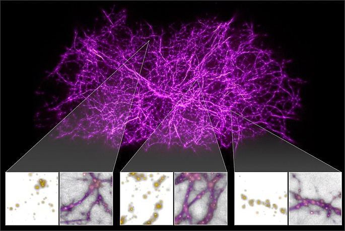
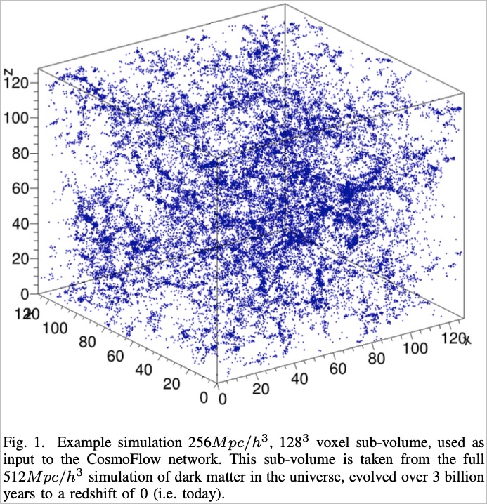
In Mathuriya[2] In their research (2018), in addition to generating cosmic data containing dark matter, they also designed a method to generate data that could be used in HPC (High-Performance Computing)., supercomputerMachine learning algorithms running in ) are intended to leverage contemporary deep learning (Deep LearningThis technology aims to accelerate the extraction of cosmic distribution characteristics from massive amounts of data. The machine learning process uses simulated data as input and processes the parameters of the simulated data (including σ)...88 megaparsecs per hour, ΩmThe proportion of matter in the universe, N The curvature of the spatiotemporal co-movement slice is used as the prediction result. The complete concept diagram of the deep learning model is as follows:
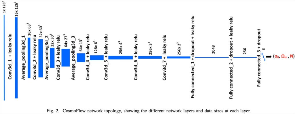
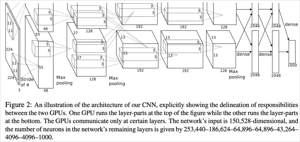
The deep model architecture shown above is a 7-layer CNN (Convolutional Neural Network)., Convolutional Neural Networks) and a fully connected 3-layer network, in conjunction with Krizhevsky, Sutskever, and Hinton (2012).[3] The proposed AlexNet architecture (see figure below) consists of a 5-layer CNN and a 3-layer fully connected network. The two are very similar, both learning the regional features of data parameters into a feature map layer through a CNN and then combining it with a fully connected network to predict the learning results.
However, for machine learning problems involving cosmological simulation data, in order to efficiently learn from large amounts of data, Mathuriya...[2]Others (2018) focused more on how to fully utilize the parallel computing resources of HPC to accelerate the learning efficiency of the system, and related strategies included using Intel®-provided... MKL-DNN, NVIDIA's cuDNN® and NCCL The kit was developed to achieve highly efficient experiments. To accelerate the computational efficiency of such large-scale cosmological machine learning, a team comprised of universities and supercomputing centers from multiple countries... ML Commons®The group is Mathuriya[2] Based on the research of [authors' names] (2018), and with the ability to accelerate the 20 days mentioned in the original study to 8.04 minutes (approximately 3,600 times faster), HPC computing facilities will be a powerful experimental tool for the study of celestial bodies.
deepDegree-based learning algorithms can be applied to cosmological simulation experiments.
Available through AI-HPC computing facilities 3,600 The experiment is accelerated by several times.
Large-scale deep learning for manipulating cosmological simulation data
forTo enable readers to practically operate machine learning based on cosmological simulation data, we provide operational details for reference by Mathuriya.[2]Research by [Authors' Name] et al. (2018) on deep learning on the CosmoFlow simulation dataset. This workflow also aims to provide a general understanding of how HPC can achieve a 3600x acceleration of artificial intelligence algorithms. The TWCC service includes Taiwan's largest and world-class supercomputer – Taiwania 2This operation is performed in Taiwania 2 This will be conducted in an environment where... All are welcome to participate.try out.
Obtain the CosmoFlow data set
The CosmoFlow simulation dataset can be found directly on the NERSC project website (https://portal.nersc.gov/project/m3363/(through) wget Command acquisition process can be found in Guy Rutenbert's documentation.[4] Operational suggestions. However, when acquiring such a large amount of data, unstable network conditions on your personal computer often lead to incomplete or missing downloads, requiring you to resume or re-upload. Therefore, we recommend logging in with your Google account. globus In order to obtain research data.
Practical application: Obtaining information
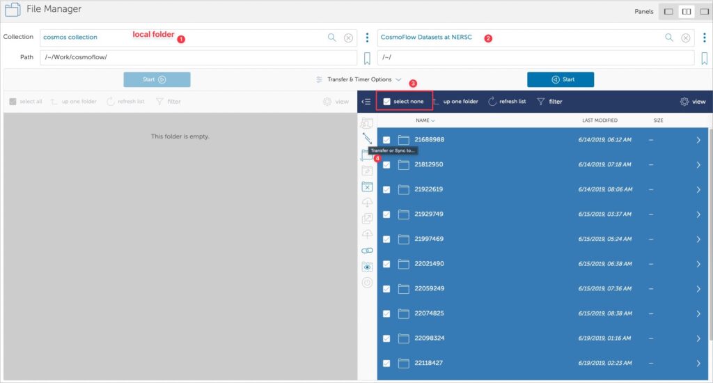
Globus is a research data sharing platform. Before downloading research materials, you need to install Globus.“Globus Connect Personal”"Software to ensure the accuracy and completeness of the research data obtained."

💁♂️ If you are using TWCC's HPC service, please confirm your account details before downloading. HFS High-Speed File System It has been set to the appropriate size and throughCheck HFS storage space usage There is still space available to avoid problems in later operations.
After downloading the dataset, you can begin deep learning training on a small-scale cosmological simulation dataset.
Experimental Procedure
Step 1. Obtain the algorithm code
Follow ML Commons® PlaceProvided deep learning algorithmsWe can begin training deep learning on small datasets of simulated universe data. However, the source code provides a version... b21518c We found some program errors in this version and suggest fixing them. The corresponding patch file is as follows:
Please obtain it yourself. b21518c Version of the code.
diff --git a/train.py b/train.py index 1a375fc..b67bed4 100644 --- a/train.py +++ b/train.py @@ -44,7 +44,7 @@ import tensorflow as tf os.environ['TF_CPP_MIN_LOG_LEVEL'] = '3' tf.compat.v1.logging.set_verbosity(logging.ERROR) import horovod.tensorflow.keras as hvd -import wandb +#import wandb # MLPerf logging try: @@ -71,7 +71,7 @@ def parse_args(): """Parse command line arguments""" parser = argparse.ArgumentParser('train.py') add_arg = parser.add_argument - add_arg('config', nargs='?', default='configs/cosmo.yaml') + add_arg('--config', nargs='?', default='configs/cosmo.yaml') add_arg('--output-dir', help='Override output directory') add_arg('--run-tag', help='Unique run tag for logging') @@ -228,7 +228,7 @@ def main(): logging.info('Configuration: %s', config) # Random seeding - tf.keras.utils.set_random_seed(args.seed) + #tf.keras.utils.set_random_seed(args.seed)
The patch documentation above mainly corrects several points.
- Remove
wandbFunction library.wandbTo facilitate the visualization of model weights and preference parameters, this work will not delve into the discussion of weights and preference parameters in deep learning models; therefore, it is recommended to remove this function. configAdding parameters--Maintain parameter consistency.- Remove random seed
set_random_seedsettings.
Step 2. In HPC environmentsRunning deep learning
In order to conduct deep learning experiments using a cosmological simulation dataset via HPC, we first need to define a training workfile, which we will refer to here as... job.sh.
For details on running HPC in TWCC, please refer to [link/reference]. HPC High-Speed Computing Tasks More information can be found in the document.
#!/bin/bash #BATCH -J MLPerf_HPC # Task Name #SBATCH -o slurm-%j.out # Output Log File Location #SBATCH --account=######### # TWCC Project id #SBATCH --nodes=2 # Number of Worker Nodes to Use #SBATCH --ntasks-per-node=8 # Number of MPIs to Run per Worker #SBATCH --cpus-per-task=4 # Number of CPUs to Use per Worker #SBATCH --gres=gpu:8 # Number of GPUs to Use per Worker #SBATCH --partition=gp1d module purge module load compiler/gnu/7.3.0 openmpi3 export NCCL_DEBUG=INFO export PYTHONFAULTHANDLER=1 export TF_ENABLE_AUTO_MIXED_PRECISION=0 SIF=/work/TWCC_cntr/tensorflow_22.01-tf2-py3.sif SINGULARITY="singularity run --nv $SIF" cmd="python train.py --config configs/cosmo_small.yaml -d --rank-gpu $@" mpirun $SINGULARITY $cmd
In the configuration script above, we defined the relevant content for this task, which includes three parts:
- L1~L9 are parameters for cross-node operation. In this example, it is set to 2 working nodes, totaling 16 GPUs.
- L11~L21 are for setting the software module and environment parameters. L19 is for using TWCC pre-configured settings.
tensorflow_22.01-tf2-py3SINGULARITY Container working environment. The HPC container environment in TWCC is a collaborative effort with NVIDIA targeting... Taiwania 2 A specially designed, optimized container runtime environment is available for users to use. - L22 is used for running large-scale computational tasks.
Before the above script is actually run, a deep learning model definition file still needs to be provided. configs/cosmo_small.yaml, where it is set as
# This YAML file describes the configuration for the MLPerf HPC v0.7 reference. output_dir: results/cosmo-000 mlperf: org: LBNL division: closed status: onprem platform: SUBMISSION_PLATFORM_PLACEHOLDER data: name: cosmo data_dir: /home/{TWCC_USRNAME}/data/cosmoflow/cosmoUniverse_2019_05_4parE_tf_small n_train: 32 n_valid: 32 sample_shape: [128, 128, 128, 4] batch_size: 4 n_epochs: 128 shard: True apply_log: True prefetch: 4 model: name: cosmoflow input_shape: [128, 128, 128, 4] target_size: 4 conv_size: 32 fc1_size: 128 fc2_size: 64 hidden_activation: LeakyReLU pooling_type: MaxPool3D dropout: 0.5 optimizer: name: SGD momentum: 0.9 lr_schedule: # Standard linear LR scaling configuration, tested up to batch size 1024 base_lr: 0.001 scaling: linear base_batch_size: 64 # Alternate # Eg if training batch size 64 you may want to adjust these decay epochs depending on your batch size. sqrt LR scaling which has worked well for batch size 512-1024. want to decay at 16 and 32 epochs. decay_schedule: 32: 0.25 64: 0.125 train: loss: mse metrics: ['mean_absolute_error'] # Uncomment to stop at target quality #target_mae: 0.124
The above deep learning model definition file configs/cosmo_small.yamlThere are many adjustable parameters, including:
- L3 output location
- Data sets L11~L21: Source and related parameters. These need to be set here.
data_dirYou must navigate to the location of the downloaded universe simulation dataset to run it successfully. - L23~L32 are model configuration files.
- L34~L36 are the optimization algorithm and its parameters.
- L38~L55 Learning Rate Hyperparameter Setting Area.
- L57~L59 Define the Loss function and stopping conditions (if needed)
After completing the settings, you can use commands to... job.sh Submit to Taiwania 2 The operation is performed using the following instructions:
sbatch job.sh
Comparison of accelerated results in large-scale experiments
Through the explanation in the previous section, I believe everyone can use it. Taiwania 2 Supercomputers are used for large-scale deep learning on cosmological simulation data, and experiments can be performed with optimal (shortest) time under different parameters and deep learning frameworks. Here, we also share the comparative results of several experimental works, including those using different versions of deep learning (…).Tensorflow, MxNet) with different numbers of GPUs and different dataset versions (CosmoFlow Data Set The cross-node training comparison between v0.7 and v1.0 is shown in the following figure:
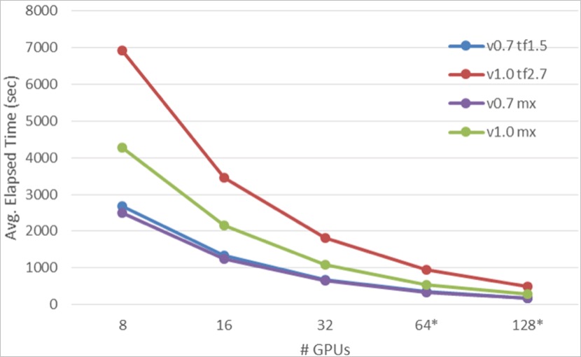
In the graph above, the Y-axis represents runtime (Time to Mean average error 0.124), and the X-axis represents the number of GPUs across nodes. The curves with lower average runtimes indicate higher efficiency. Experimental data shows... MxNet (Green and purple) are both higher than Tensorflow (Blue, Red) in different versions CosmoFlow Data SetIt is relatively efficient. We infer this is because... MxNet The dataset has already been decompressed in the preprocessing stage, and... Tensorflow Decompression occurs only at runtime during computation. Further discussion of the acceleration effect across nodes is illustrated in the table below:
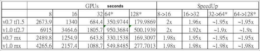
Large-scale deep learning experiments using cosmological simulation data show that each additional computing node (Taiwania 2 A single computing node (consisting of 8 V100 GPUs) can improve computing efficiency by approximately 2 times and reduce computing time costs by approximately 14.7 times. This not only improves the efficiency of obtaining results from experimental hypotheses but also makes space research outputs more fruitful.
Furthermore, due to Taiwania 2 For HPC environments that are ready-to-use and provide ample GPU computing resources for Chinese users, overall computing costs can be more effectively controlled under on-demand computing cost calculations. This is based on the large-scale deep learning experimental data mentioned above. Tensorflow study CosmoFlow Data Set The following analysis uses the calculation data from v0.7:
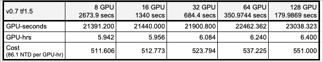
As shown in the table above, to accelerate the acquisition of experimental results, we increased the cross-node computing scale from the original 8 GPUs (1 compute node) to 128 GPUs (16 compute nodes). While the overall computing cost only increased from 511 NTD to 551 NTD, the computing efficiency was indeed accelerated by 14.7 times. Without modifying any algorithm computing logic or the computing environment, the artificial intelligence algorithm can achieve [the following]: Taiwania 2 The computing facility directly accelerates experimental efficiency and effectively controls experimental costs.
Taiwania2 Allowing users to perform without modifying any algorithm,
Improve computational efficiency by approximately14.7 times.
Conclusion
This article explains how to... N-body simulation In performing cosmological calculations, besides proposing several celestial models, the paper also introduces methods for incorporating more astrophysical assumptions into these models. Contemporary computer science scholar Mathuriya...[2] et al. (2018) proposed a machine learning architecture for cosmological simulation data using large-scale deep learning, and accelerated the acquisition of hypothesis verification data through an HPC environment. In Mathuriya...[2] In the study by Krizhevsky et al. (2012), reference was made to Krizhevsky et al. (2012).[3] The proposed AlexNet architecture and its algorithmic model enable deep learning algorithms to learn from simulated celestial data containing dark matter. The overall experimental process was also conducted through…ML Commons®The team reduced the overall computation time from 20 days to 8.04 minutes (approximately 3600 times faster). Finally, we also explain the supercomputer built with funding from the Republic of China government. Taiwania 2 How to perform Mathuriya[2] The research by et al. (2018), in addition to comparing the computational efficiency of different deep learning frameworks, also illustrates that...Taiwania 2 Using large-scale deep learning computing can directly achieve the benefits of high-speed computing at virtually zero cost (without modifying the code or the computing framework).
Those interested in astronomical research may also visit TWCC of Taiwania 2 Conduct various interesting celestial experiments!
References
GitHub Project Josephbakulikira/N-body-simulation-with-python–Gravity-solar-system
Mathuriya, A., Bard, D., Meadows, L., et. al., “CosmoFlow: Using Deep Learning to Learn the Universe at Scale,” SC18, November 11-16, 2018, Dallas, Texas, USA. https://arxiv.org/abs/1808.04728
Krizhevsky, A., Sutskever, I., & Hinton, GE (2012). Imagenet classification with deep convolutional neural networks. Advances in neural information processing systems, 25.
Guy Rutenberg, “Make Offline Mirror of a Site using
wget”, https://www.guyrutenberg.com/2014/05/02/make-offline-mirror-of-a-site-using-wget/